Causal forecasting with regression
Annoyingly have to print all the code together becuase they don’t want to use ggplot…
Some more complex data, data with spikes that might be caused by promotions:
setwd("/Users/rosseji/Dropbox/TrendLock/ISF/forecasting with R/")
sales <- scan("sales.txt")
# Plot the sales as a line
plot(sales, type="l", xlab="Weeks", ylab="Sales")
# Save the length of the sales into a variable
n <- length(sales)
# Scan the promotional data and save into a data frame
promos <- data.frame(promo1=scan("promo1.txt"), promo2=scan("promo2.txt"), promo3=scan("promo3.txt"))
# Diplay the data frame in the console
head(promos)
## promo1 promo2 promo3
## 1 0 0 0
## 2 0 0 0
## 3 0 0 0
## 4 0 0 1
## 5 0 0 1
## 6 0 0 0# Save the length of the information regarding forthcoming promotional activity (or forecasting horizon)
h <- nrow(promos)-n
# Plot the promotional activity information on the existing plot
points(which(promos[,1]==1), sales[which(promos[,1]==1)], pch=1, col="blue", cex=1.5, lwd=2)
points(which(promos[,2]==1), sales[which(promos[,2]==1)], pch=2, col="red", cex=1.5)
points(which(promos[,3]==1), sales[which(promos[,3]==1)], pch=3, col="orange", cex=1)
# Fit an additive regression model
fit1 <- lm(sales ~ promo1 + promo2 + promo3, promos[1:n,])
# Return the summary of the model
summary(fit1)##
## Call:
## lm(formula = sales ~ promo1 + promo2 + promo3, data = promos[1:n,
## ])
##
## Residuals:
## Min 1Q Median 3Q Max
## -483.44 -120.07 -7.94 120.73 613.04
##
## Coefficients:
## Estimate Std. Error t value Pr(>|t|)
## (Intercept) 943.13 22.18 42.516 <2e-16 ***
## promo1 758.52 60.92 12.450 <2e-16 ***
## promo2 1166.43 58.05 20.095 <2e-16 ***
## promo3 58.30 36.31 1.605 0.112
## ---
## Signif. codes: 0 '***' 0.001 '**' 0.01 '*' 0.05 '.' 0.1 ' ' 1
##
## Residual standard error: 168.5 on 92 degrees of freedom
## Multiple R-squared: 0.8882, Adjusted R-squared: 0.8845
## F-statistic: 243.6 on 3 and 92 DF, p-value: < 2.2e-16# Add a new line (the fit of the model) on the existing graph
lines(fit1$fit, col="blue")
# Create lagged variables of the promotions
promos_lag <- rbind(c(0,0,0), promos)
names(promos_lag) <- c("promo1_lag", "promo2_lag", "promo3_lag")
# Combine the two data frames
promos <- cbind(promos, promos_lag[1:(n+h),])
# Diplay the expanded data frame in the console
head(promos)## promo1 promo2 promo3 promo1_lag promo2_lag promo3_lag
## 1 0 0 0 0 0 0
## 2 0 0 0 0 0 0
## 3 0 0 0 0 0 0
## 4 0 0 1 0 0 0
## 5 0 0 1 0 0 1
## 6 0 0 0 0 0 1# Fit an additive regression model, adding the lagged effects of the promotions
fit2 <- lm(sales ~ promo1 + promo2 + promo3 + promo1_lag + promo2_lag + promo3_lag, promos[1:n,])
# Return the summary of the model
summary(fit2) ##
## Call:
## lm(formula = sales ~ promo1 + promo2 + promo3 + promo1_lag +
## promo2_lag + promo3_lag, data = promos[1:n, ])
##
## Residuals:
## Min 1Q Median 3Q Max
## -263.72 -60.76 -7.54 54.53 540.79
##
## Coefficients:
## Estimate Std. Error t value Pr(>|t|)
## (Intercept) 1012.32 16.59 61.037 < 2e-16 ***
## promo1 793.74 42.39 18.723 < 2e-16 ***
## promo2 1134.28 40.67 27.892 < 2e-16 ***
## promo3 176.56 28.79 6.134 2.32e-08 ***
## promo1_lag -71.48 42.72 -1.673 0.097799 .
## promo2_lag -148.01 40.00 -3.700 0.000373 ***
## promo3_lag -255.06 29.04 -8.783 1.06e-13 ***
## ---
## Signif. codes: 0 '***' 0.001 '**' 0.01 '*' 0.05 '.' 0.1 ' ' 1
##
## Residual standard error: 114.6 on 89 degrees of freedom
## Multiple R-squared: 0.95, Adjusted R-squared: 0.9466
## F-statistic: 281.9 on 6 and 89 DF, p-value: < 2.2e-16# Add a new line (the fit of the model) on the existing graph
lines(fit2$fit, col="green") 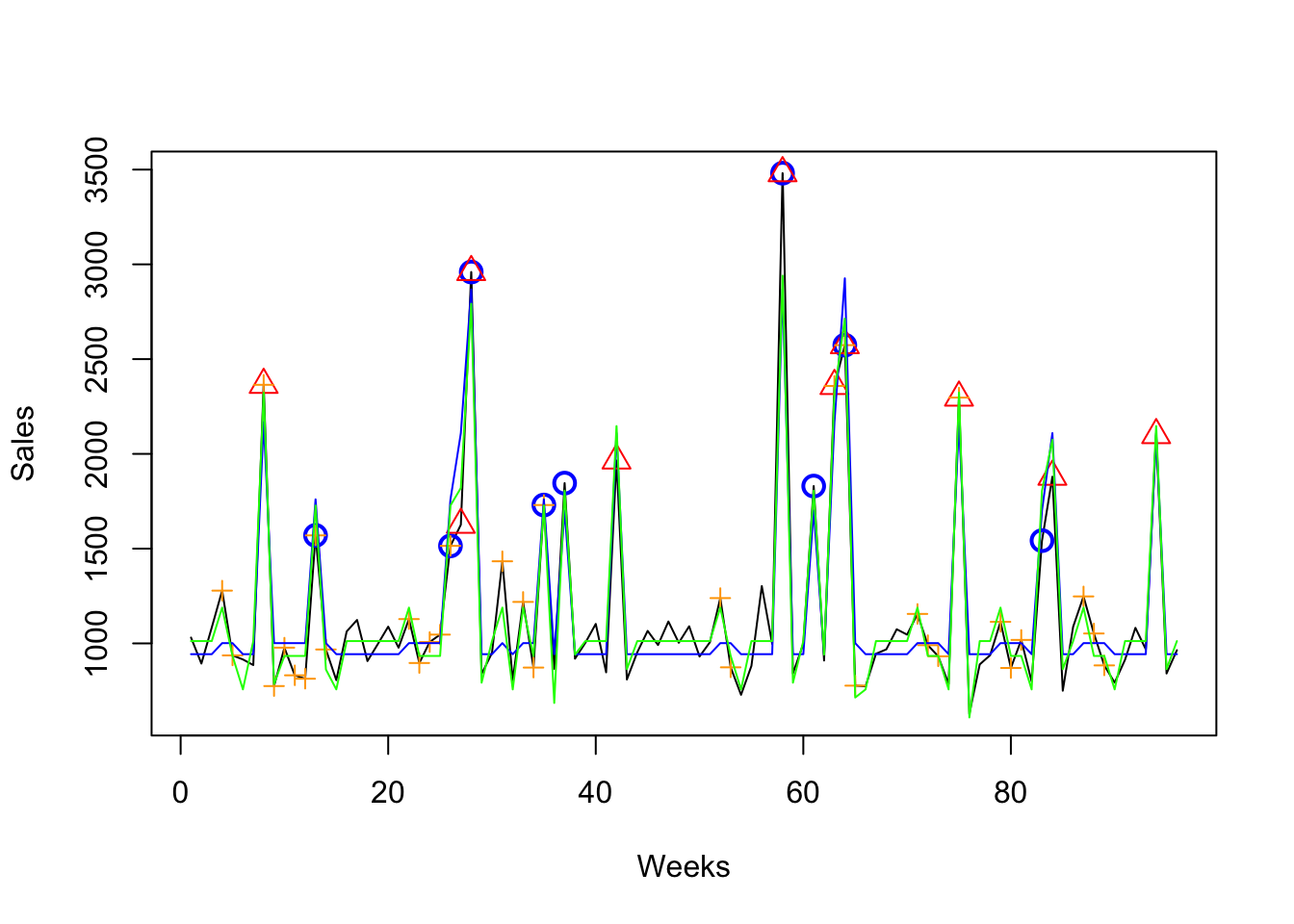
# Calculate the out-of-sample forecasts, based on the available information on forthcoming promotions
fcs <- predict(fit2, promos[(n+1):(n+h),])
fcs
## 97 98 99 100 101 102 103
## 2146.5950 1040.8702 757.2550 1012.3163 1188.8804 933.8191 933.8191
## 104 105 106 107 108 109
## 757.2550 1012.3163 1188.8804 2068.0978 609.2449 1012.3163# Plot the sales as a line
plot(sales, type="l", xlab="Weeks", ylab="Sales", xlim=c(1,109))
# Plot the forecasts as a new line
lines(x=(n+1):(n+h), fcs, col="blue")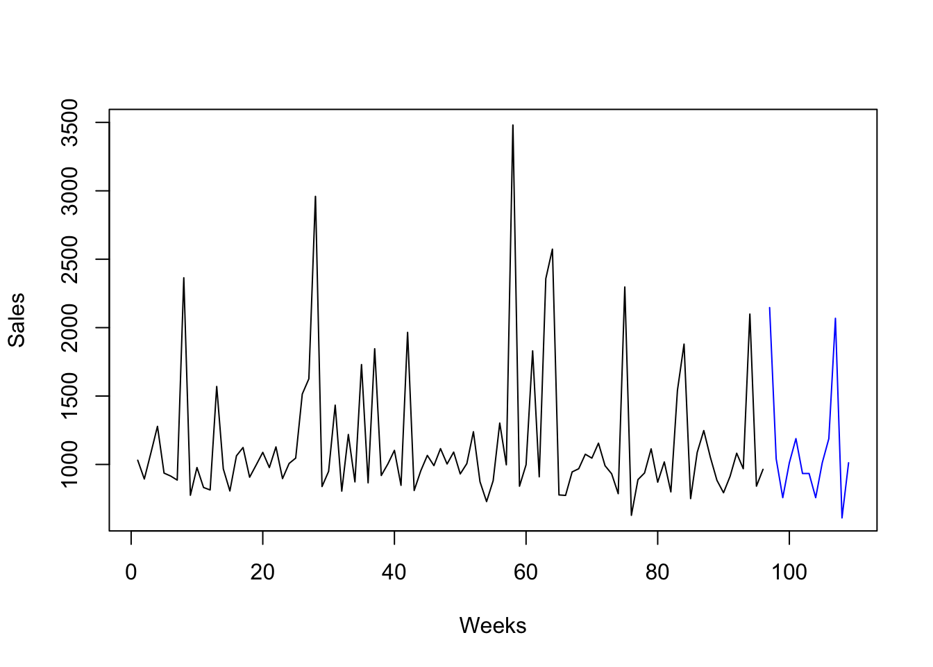
# Calculate the natural logarithm of the sales
logsales <- log(sales)
# Fit a regression model
fitlog <- lm(logsales ~ promo1 + promo2 + promo3 + promo1_lag + promo2_lag + promo3_lag, promos[1:n,])
# Return the summary of the model
summary(fitlog)
##
## Call:
## lm(formula = logsales ~ promo1 + promo2 + promo3 + promo1_lag +
## promo2_lag + promo3_lag, data = promos[1:n, ])
##
## Residuals:
## Min 1Q Median 3Q Max
## -0.167208 -0.054359 -0.003812 0.050412 0.262658
##
## Coefficients:
## Estimate Std. Error t value Pr(>|t|)
## (Intercept) 6.909358 0.011253 614.012 < 2e-16 ***
## promo1 0.545815 0.028762 18.977 < 2e-16 ***
## promo2 0.689956 0.027591 25.007 < 2e-16 ***
## promo3 0.172585 0.019531 8.837 8.19e-14 ***
## promo1_lag -0.003724 0.028983 -0.128 0.898
## promo2_lag -0.201535 0.027139 -7.426 6.44e-11 ***
## promo3_lag -0.235294 0.019703 -11.942 < 2e-16 ***
## ---
## Signif. codes: 0 '***' 0.001 '**' 0.01 '*' 0.05 '.' 0.1 ' ' 1
##
## Residual standard error: 0.07774 on 89 degrees of freedom
## Multiple R-squared: 0.9475, Adjusted R-squared: 0.944
## F-statistic: 268 on 6 and 89 DF, p-value: < 2.2e-16# Plot the sales as a line
plot(sales, type="l", lwd=2)
# Add a line for the fitted values (which are transformed using the exponential function)
lines(exp(fitlog$fit), col="orange")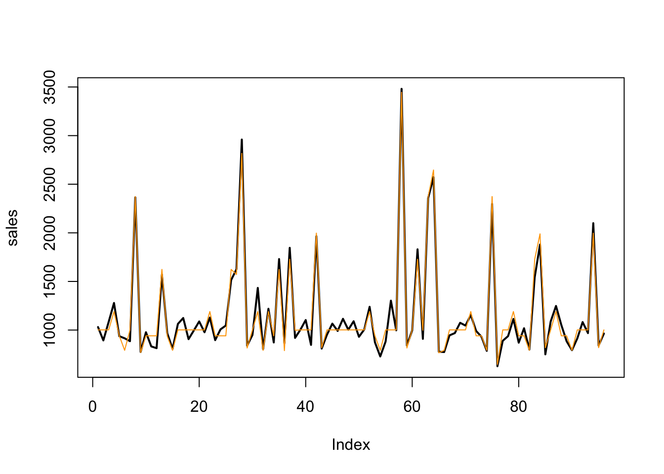
# ----- Selecting independent variables -----
# Backwards stepwise regression
step(lm(sales ~ promo1 + promo2 + promo3 + promo1_lag + promo2_lag + promo3_lag, promos[1:n,]))
## Start: AIC=917.06
## sales ~ promo1 + promo2 + promo3 + promo1_lag + promo2_lag +
## promo3_lag
##
## Df Sum of Sq RSS AIC
## <none> 1168490 917.06
## - promo1_lag 1 36756 1205246 918.03
## - promo2_lag 1 179758 1348247 928.80
## - promo3 1 493934 1662424 948.91
## - promo3_lag 1 1012860 2181349 974.99
## - promo1 1 4602607 5771096 1068.39
## - promo2 1 10214283 11382772 1133.59##
## Call:
## lm(formula = sales ~ promo1 + promo2 + promo3 + promo1_lag +
## promo2_lag + promo3_lag, data = promos[1:n, ])
##
## Coefficients:
## (Intercept) promo1 promo2 promo3 promo1_lag
## 1012.32 793.74 1134.28 176.56 -71.48
## promo2_lag promo3_lag
## -148.01 -255.06Notice the effecct of being able to lag the the target variables to check for the delayed effect of worse sales!