Intermittent demand forecasting
Like… Slow moving items, like bottles of wine?
setwd("/Users/rosseji/Dropbox/TrendLock/ISF/forecasting with R/")
ts1.test <- ts(scan("ts1out.txt"), start=c(2016,1), frequency=4)
ts2.test <- ts(scan("ts2out.txt"), start=c(2016,1), frequency=12)

# Load the necessary library
library(tsintermittent)
## Loading required package: MAPA## Loading required package: forecast## Loading required package: parallel## Loading required package: RColorBrewer## Loading required package: smooth## This is package "smooth", v1.9.9# Load the third time series
y <- ts(scan("ts3.txt"), start=c(2011,1), frequency=12)
y.test <- ts(scan("ts3out.txt"), start=c(2016,1), frequency=12)
# Set the forecats horizon to be equal to the test set
h <- length(y.test)
# First we plot the series to get a general impression
plot(y)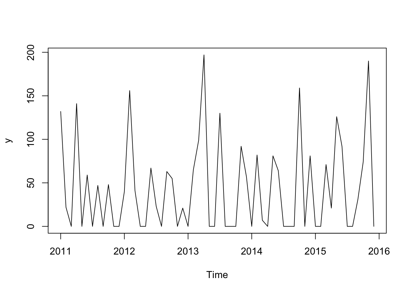
# Croston's method
f.crost <- crost(y,h=h,outplot=1)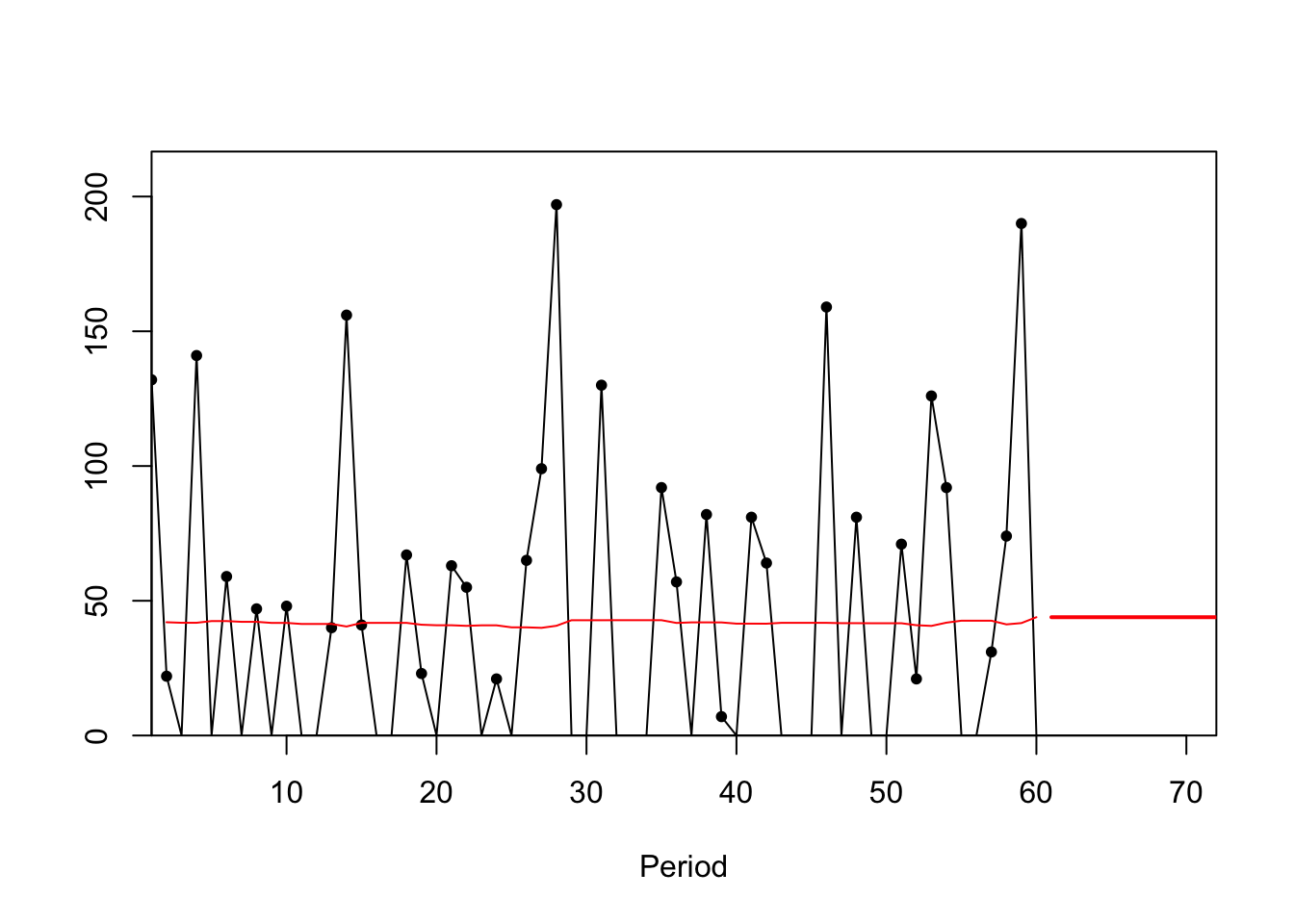
# The output contains various results which are documented in the function help.
print(f.crost)
## $model
## [1] "croston"
##
## $frc.in
## [1] NA 42.03016 41.83333 41.83333 42.46275 42.46275 42.18760
## [8] 42.18760 41.78218 41.78218 41.39217 41.39217 41.39217 40.44976
## [15] 41.78823 41.79557 41.79557 41.79557 41.11239 40.91241 40.91241
## [22] 40.69247 40.88418 40.88418 40.13630 40.13630 39.95113 40.72067
## [29] 42.77451 42.77451 42.77451 42.79148 42.79148 42.79148 42.79148
## [36] 41.77028 41.98360 41.98360 41.96318 41.51184 41.51184 41.48936
## [43] 41.81276 41.81276 41.81276 41.81276 41.68598 41.68598 41.65861
## [50] 41.65861 41.65861 40.93039 40.67289 41.87612 42.60286 42.60286
## [57] 42.60286 41.23357 41.71786 43.90001
##
## $frc.out
## [1] 43.90001 43.90001 43.90001 43.90001 43.90001 43.90001 43.90001
## [8] 43.90001 43.90001 43.90001 43.90001 43.90001
##
## $weights
## [1] 0.03292563 0.03351995
##
## $initial
## [1] 132.393905 3.149974
##
## $components
## $components$c.in
## Demand Interval
## [1,] NA NA
## [2,] 132.39391 3.149974
## [3,] 128.75912 3.077907
## [4,] 128.75912 3.077907
## [5,] 129.16216 3.041776
## [6,] 129.16216 3.041776
## [7,] 126.85202 3.006855
## [8,] 126.85202 3.006855
## [9,] 124.22284 2.973106
## [10,] 124.22284 2.973106
## [11,] 121.71316 2.940487
## [12,] 121.71316 2.940487
## [13,] 121.71316 2.940487
## [14,] 119.02270 2.942482
## [15,] 120.24020 2.877370
## [16,] 117.63117 2.814441
## [17,] 117.63117 2.814441
## [18,] 117.63117 2.814441
## [19,] 115.96410 2.820661
## [20,] 112.90320 2.759632
## [21,] 112.90320 2.759632
## [22,] 111.26011 2.734169
## [23,] 109.40771 2.676040
## [24,] 109.40771 2.676040
## [25,] 106.49683 2.653379
## [26,] 106.49683 2.653379
## [27,] 105.13052 2.631478
## [28,] 104.92867 2.576791
## [29,] 107.96018 2.523937
## [30,] 107.96018 2.523937
## [31,] 107.96018 2.523937
## [32,] 108.68585 2.539895
## [33,] 108.68585 2.539895
## [34,] 108.68585 2.539895
## [35,] 108.68585 2.539895
## [36,] 108.13646 2.588837
## [37,] 106.45276 2.535580
## [38,] 106.45276 2.535580
## [39,] 105.64764 2.517627
## [40,] 102.39960 2.466756
## [41,] 102.39960 2.466756
## [42,] 101.69500 2.451111
## [43,] 100.45387 2.402469
## [44,] 100.45387 2.402469
## [45,] 100.45387 2.402469
## [46,] 100.45387 2.402469
## [47,] 102.38154 2.456019
## [48,] 102.38154 2.456019
## [49,] 101.67754 2.440733
## [50,] 101.67754 2.440733
## [51,] 101.67754 2.440733
## [52,] 100.66746 2.459479
## [53,] 98.04436 2.410558
## [54,] 98.96482 2.363276
## [55,] 98.73550 2.317579
## [56,] 98.73550 2.317579
## [57,] 98.73550 2.317579
## [58,] 96.50526 2.340454
## [59,] 95.76426 2.295522
## [60,] 98.86703 2.252096
##
## $components$c.out
## Demand Interval
## [1,] 98.86703 2.252096
## [2,] 98.86703 2.252096
## [3,] 98.86703 2.252096
## [4,] 98.86703 2.252096
## [5,] 98.86703 2.252096
## [6,] 98.86703 2.252096
## [7,] 98.86703 2.252096
## [8,] 98.86703 2.252096
## [9,] 98.86703 2.252096
## [10,] 98.86703 2.252096
## [11,] 98.86703 2.252096
## [12,] 98.86703 2.252096
##
## $components$coeff
## [1] 1# $frc.out is the out-of-sample forecast so we will retain only this
f.crost <- f.crost$frc.out